Tutorials

Introduction

kmcos is designed for lattice based Kinetic Monte Carlo simulations to understand chemical kinetics and mechanisms. It has been used to produce more than 10 scientific publications. The best way to learn how to use kmcos is by following the examples.

If you have already followed the kmcos installation instructions and still have the kmcosInstallation directory, then navigate to /kmcosInstallation/kmcos/examples

If you do not have that directory, but have kmcos installed, go to https://github.com/kmcos/kmcos Click on the green button and download zip, to get the examples.

Inside /examples/, run the following commands

python3 MyFirstSnapshots__build.py
cd MyFirstSnapshots_local_smart
python3 runfile.py

The first command uses a python file to create a chemical model (process definitions) and a KMC modeling executable as well. The “local_smart” is the default backend (default “KMC Engine”, kmcos has several).

After the simulation has run, you will see a csv file named runfile_TOFs_and_Coverages.csv, open this file to see your first KMC output!

Various examples exist. More features and a thorough tutorial are forthcoming. Please join the kmcos-users group https://groups.google.com/g/kmcos-users and email any questions if you get stuck.

Feature overview

This paragraph is from __init__.py

With kmcos you can:

• easily create and modify kMC models through GUI
• store and exchange kMC models through XML
• generate fast, platform independent, self-contained code [1]
• run kMC models through GUI or python bindings

kmcos has been developed in the context of first-principles based modelling of surface chemical reactions but might be of help for other types of kMC models as well.

kmcos’ goal is to significantly reduce the time you need to implement and run a lattice kmc simulation. However it can not help you plan the model.

Typical users will run kmcos entirely from python code by following the examples.

Footnotes

[1]	The source code is generated in Fortran90, written in a modular fashion. Python bindings are generated using f2py.

The Runtime View

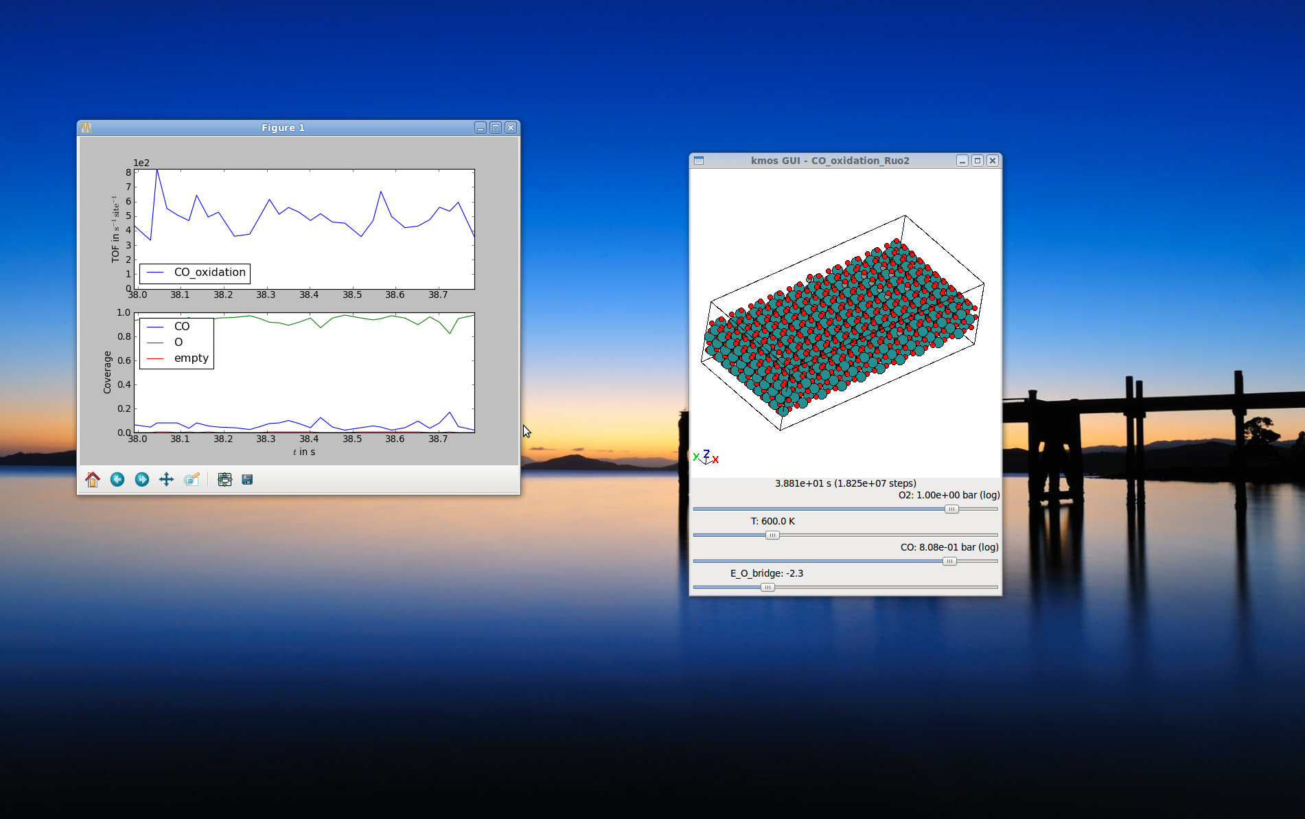
The compiled module can be run and watched in realtime. When parameters are changed this is immediately reflected in the rate constants.

A first kMC Model–the API way

In general there are two interfaces to defining a new model: A GUI and an API. While the GUI can be quite nice especially for beginners, it turns out that the API is better maintained simply because … well, maintaing a GUI is a lot more work.

So we will start by learning how to setup the model using the API which will turn out not to be hard at all. It is knowing howto do this will also pay-off especially if you starting tinkering with your existing models and make little changes here and there.

Build the model

You may also look at MyFirstDiffusion__build.py in the examples directory.

We start by making the necessary import statements (in *python* or better *ipython*):

import kmcos
from kmcos.types import *
from kmcos.io import *
import numpy as np

which imports all classes that make up a kMC project. The functions from kmcos.io will only be needed at the end to save the project or to export compilable code.

The example sketched out here leads you to a kMC model for CO adsorption and desorption on Pd(100). First you should instantiate a new project and fill in meta information

kmc_model = kmcos.create_kmc_model()
kmc_model.set_meta(author = 'Your Name',
            email = 'your.name@server.com',
            model_name = 'MyFirstModel',
            model_dimension = 2,)

Next you add some species or states. Note that whichever species you add first is the default species with which all sites in the system will be initialized. Of course this can be changed later

For surface science simulations it is useful to define an empty state, so we add

kmc_model.add_species(name='empty')

and some surface species. Given you want to simulate CO adsorption and desorption on a single crystal surface you would say

kmc_model.add_species(name='CO',
               representation="Atoms('CO',[[0,0,0],[0,0,1.2]])")

where the string passed as representation is a string representing a CO molecule which can be evaluated in ASE namespace.

Once you have all species declared is a good time to think about the geometry. To keep it simple we will stick with a simple-cubic lattice in 2D which could for example represent the (100) surface of a fcc crystal with only one adsorption site per unit cell. You start by giving your layer a name

layer = kmc_model.add_layer(name='simple_cubic')

and adding a site

layer.sites.append(Site(name='hollow', pos='0.5 0.5 0.5',
                        default_species='empty'))

Where pos is given in fractional coordinates, so this site will be in the center of the unit cell.

Simple, huh? Now you wonder where all the rest of the geometry went? For a simple reason: the geometric location of a site is meaningless from a kMC point of view. In order to solve the master equation none of the numerical coordinates of any lattice sites matter since the master equation is only defined in terms of states and transition between these. However to allow a graphical representation of the simulation one can add geometry as you have already done for the site. You set the size of the unit cell via

kmc_model.lattice.cell = np.diag([3.5, 3.5, 10])

which are prototypical dimensions for a single-crystal surface in Angstrom.

Ok, let us see what we managed so far: you have a lattice with a site that can be either empty or occupied with CO.

Populate process list and parameter list

The remaining work is to populate the process list and the parameter list. The parameter list defines the parameters that can be used in the expressions of the rate constants. In principle one could do without the parameter list and simply hard code all parameters in the process list, however one looses some nifty functionality like easily changing parameters on-the-fly or even interactively.

A second benefit is that you achieve a clear separation of the kinetic model from the barrier input, which usually has a different origin.

In practice filling the parameter list and the process list is often an iterative process, however since we have a fairly short list, we can try to set all parameters at once.

First of all you want to define the external parameters to which our model is coupled. Here we use the temperature and the CO partial pressure:

kmc_model.add_parameter(name='T', value=600., adjustable=True, min=400, max=800)
kmc_model.add_parameter(name='p_CO', value=1., adjustable=True, min=1e-10, max=1.e2)

You can also set a default value and a minimum and maximum value set defines how the scrollbars a behave later in the runtime GUI.

To describe the adsorption rate constant you will need the area of the unit cell:

kmc_model.add_parameter(name='A', value='(3.5*angstrom)**2')

Last but not least you need a binding energy of the particle on the surface. Since without further ado we have no value for the gas phase chemical potential, we’ll just call it deltaG and keep it adjustable

kmc_model.add_parameter(name='deltaG', value='-0.5', adjustable=True,
                           min=-1.3, max=0.3)

To define processes we first need a coordinate [3]

coord = kmc_model.lattice.generate_coord('hollow.(0,0,0).simple_cubic')

Then you need to have at least two processes. A process or elementary step in kMC means that a certain local configuration must be given so that something can happen at a certain rate constant. In the framework here this is phrased in terms of ‘conditions’ and ‘actions’. [2] So for example an adsorption requires at least one site to be empty (condition). Then this site can be occupied by CO (action) with a rate constant. Written down in code this looks as follows

kmc_model.add_process(name='CO_adsorption',
               conditions=[Condition(coord=coord, species='empty')],
               actions=[Action(coord=coord, species='CO')],
               rate_constant='p_CO*bar*A/sqrt(2*pi*umass*m_CO/beta)')

Note

In order to ensure correct functioning of the kmcos kMC solver every action should have a corresponding condition for the same coordinate.

Now you might wonder, how come we can simply use m_CO and beta and such. Well, that is because the evaluator will to some trickery to resolve such terms. So beta will be first be translated into 1/(kboltzmann*T) and as long as you have set a parameter T before, this will go through. Same is true for m_CO, here the atomic masses are looked up and added. Note that we need conversion factors of bar and umass.

Then the desorption process is almost the same, except the reverse:

kmc_model.add_process(name='CO_desorption',
               conditions=[Condition(coord=coord, species='CO')],
               actions=[Action(coord=coord, species='empty')],
               rate_constant='p_CO*bar*A/sqrt(2*pi*umass*m_CO/beta)*exp(beta*deltaG*eV)')

To reduce typing, kmcos also knows a shorthand notation for processes. In order to produce the same process you could also type

kmc_model.parse_process('CO_desorption; CO@hollow->empty@hollow ; p_CO*bar*A/sqrt(2*pi*umass*m_CO/beta)*exp(beta*deltaG*eV)')

and since any non-existing on either the left or the right side of the -> symbol is replaced by a corresponding term with the default_species (in this case empty) you could as well type

kmc_model.parse_process('CO_desorption; CO@hollow->; p_CO*bar*A/sqrt(2*pi*umass*m_CO/beta)*exp(beta*deltaG*eV)')

and to make it even shorter you can parse and add the process on one line

kmc_model.parse_and_add_process('CO_desorption; CO@hollow->; p_CO*bar*A/sqrt(2*pi*umass*m_CO/beta)*exp(beta*deltaG*eV)')

In order to add processes on more than one site possible spanning across unit cells, there is a shorthand as well. The full-fledged syntax for each coordinate is

"<site-name>.<offset>.<lattice>"

check Manual generation for details.

Export, save, compile

Before we compile the model, we should specify and understand the various backends that are involved.

local_smart backend (default) for models with <100 processes. lat_int backend for models with >100 processes. (build the model same ways local_smart but different backend for compile step) otf backend requires custom model (build requires different process definitions compared to local_smart) and can work for models which require >10000 processes, since each process rate is calculated on the fly instead of being held in memory.

Here is how we specify the model’s backend

kmc_model.backend = 'local_smart'
kmc_model.backend = 'lat_int'
kmc_model.backend = 'otf'

Next, it’s a good idea to save and compile your work

kmc_model.save_model()
kmcos.compile(kmc_model)

This creates an XML file with the full definition of your model and exports the model to compiled code.

Now is the time to leave the python shell. In the current directory you should see a myfirst_kmc.xml. You will also see a directory ending with _local_smart, this directory includes your compiled model.

You can also skip the model exporting and do it later by removing kmcos.compile(kmc_model): you can use a separate python file later, or from the command line can run kmcos export myfirst_kmc.xml in the same directory as the XML.

During troubleshooting, exporting separately can be useful to make sure the compiling occurs gracefully without any line containining an error.

Running and viewing the model

If you now cd to that folder myfirst_kmc_local_smart and run

python3 kmc_settings.py benchmark

You should see that the model was able to run! Next, let’s try seeing how it looks visually with

python3 kmc_settings.py view

… and dada! Your first running kMC model right there! For some installations, one can type kmcos benchmark and kmcos view.

For running the model, you should use a runfile.

If you wonder why the CO molecules are basically just dangling there in mid-air that is because you have no background setup, yet. Choose a transition metal of your choice and add it to the lattice setup for extra credit :-).

Wondering where to go from here? If the work-flow makes complete sense, you have a specific model in mind, and just need some more idioms to implement it I suggest you take a look at the examples folder. for some hints. To learn more about the kmcos approach and methods you should into topic guides.

In technical terms, kmcos is run an API via the kmcos python module.

Additionally, though now discouraged, kmcos can be invoked directly from the command line in one of the following ways:

kmcos [help] (all|benchmark|build|edit|export|help|import|rebuild|run|settings-export|shell|version|view|xml) [options]

Taking it home

Despite its simplicity you have now seen all elements needed to implement a kMC model and hopefully gotten a first feeling for the workflow.

[2]	You will have to describe all processes in terms of conditions and actions and you find a more complete description in the topic guide to the process description syntax.

[3]	The description of coordinates follows the simple syntax of the coordinate syntax and the topic guide explains how that works.

An alternative way using .ini files

Presently, a full description of the .ini capability is not being provided because this way is not the standard way of using kmcos. However, it is available. This method is an alternative to making an xml file, and can be used instead of kmcos export.

Prepare a minimal input file with the following content and save it as mini_101.ini

[Meta]
author = Your Name
email = you@server.com
model_dimension = 2
model_name = fcc_100

[Species empty]
color = #FFFFFF

[Species CO]
representation = Atoms("CO", [[0, 0, 0], [0, 0, 1.17]])
color = #FF0000

[Lattice]
cell_size = 3.5 3.5 10.0

[Layer simple_cubic]
site hollow = (0.5, 0.5, 0.5)
color = #FFFFFF

[Parameter k_CO_ads]
value = 100
adjustable = True
min = 1
max = 1e13
scale = log

[Parameter k_CO_des]
value = 100
adjustable = True
min = 1
max = 1e13
scale = log

[Process CO_ads]
rate_constant = k_CO_ads
conditions = empty@hollow
actions = CO@hollow
tof_count = {'adsorption':1}

[Process CO_des]
rate_constant = k_CO_des
conditions = CO@hollow
actions = empty@hollow
tof_count = {'desorption':1}

In the same directory run kmcos export mini_101.ini. You should now have a folder mini_101_local_smart in the same directory. cd into it and run kmcos benchmark. If everything went well you should see something like

Using the [local_smart] backend.
1000000 steps took 1.51 seconds
Or 6.62e+05 steps/s

In the same directory try running kmcos view to watch the model run or fire up kmcos shell to interact with the model interactively. Explore more commands with kmcos help and please refer to the documentation how to build complex model and evaluate them systematically. To test all bells and whistles try kmcos edit mini_101.ini and inspect the model visually.

Todo

describe modelling more complicated structures and e.g. boundary conditions

The Model Editor (Deprecated – glade migration is required to revive this feature)

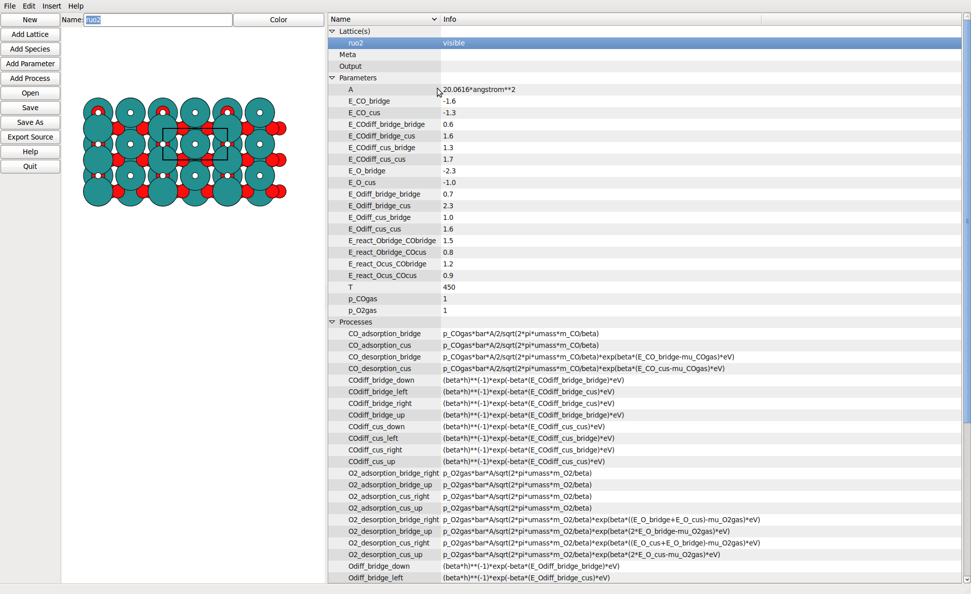
The lattice view allows to define sites by simple pointing.

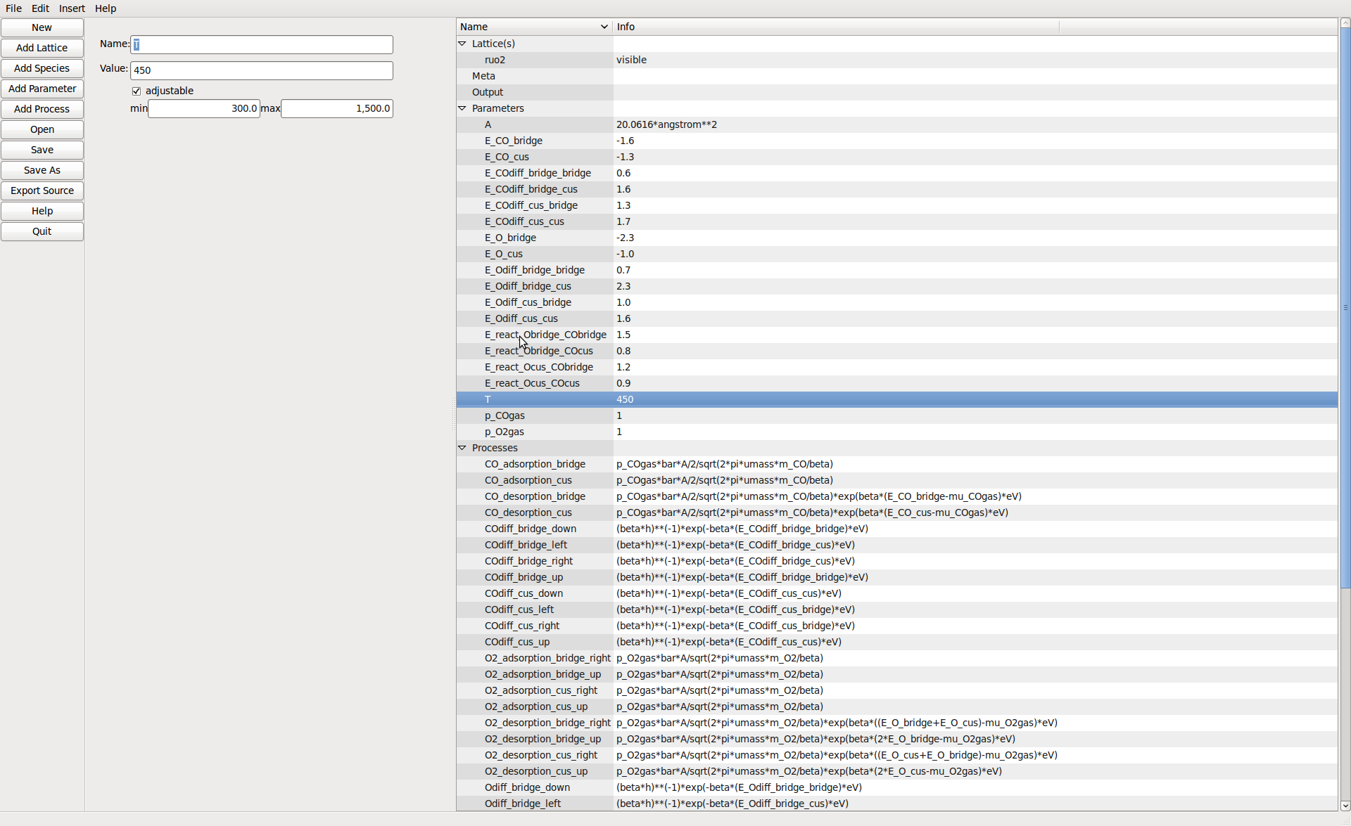
Model parameters can be defined including ranges to vary them over in the runtime viewer.

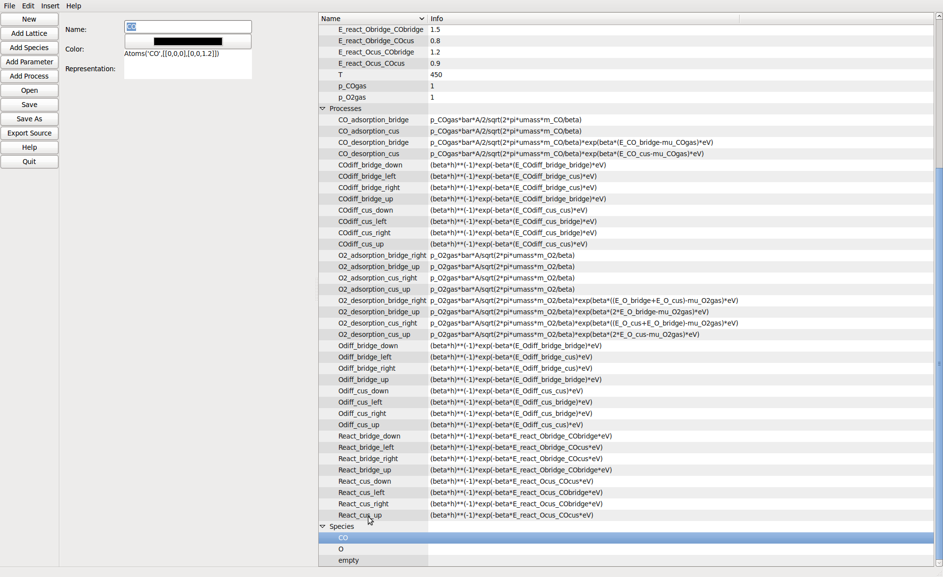
Species can be added here. The color is used to represent them in the 2D editor view. The string is an ASE atoms constructor for display at runtime.

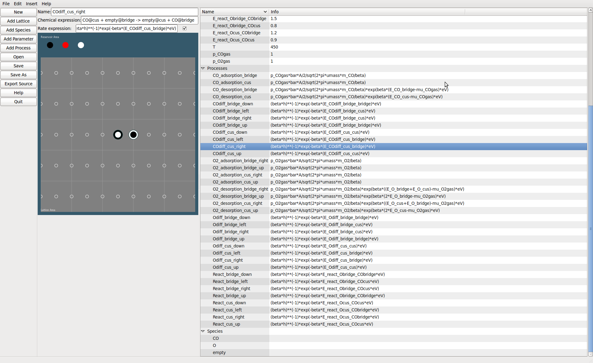
Processes can be added by point and click or by entering a chemical expression.

Running the Model From Runfiles

Running the Model–the API way

In order to analyze a model in quantitatively it is more practical to write small client scripts that directly talk to the runtime API. As time passes and more of these scripts are written over and over some standard functionality will likely be integrated into the runtime API. For starters a simple script could look as follows

#!/usr/bin/env python

from kmcos.run import KMC_Model

model = KMC_Model()

An alternative way that gets you started fast it to run

kmcos shell

and just interact directly with model. It is often a good idea to

%logstart some_scriptname.py

first in the IPython command to save what you have typed for later use.

As you can see by default the model prints a disclaimer and all rate constants, which can each be turned off by instantiating

model = KMC_Model(print_rates=False, banner=False)

The most important method is of course how to run the model, which you can do by saying

model.do_steps(100000)

which would run the model by 100,000 kMC steps.

Let’s say you want to change the temperature and a partial pressure of the model you could type

model.parameters.T = 550
model.parameters.p_COgas = 0.5

and all rate constants are instantly updated. In order get a quick overview of the current settings you can issue e.g.

print(model.parameters)
print(model.rate_constants)

or just

print(model)

Now an instantiated und configured model has mainly two functions: run kMC steps and report its current configuration.

To analyze the current state you may use

atoms = model.get_atoms()

Note

If you want to fetch data from the current state without actually visualizing the geometry can speed up the get_atoms() call using

atoms = model.get_atoms(geometry=False)

This will return an ASE atoms object of the current system, but it also contains some additional data piggy-backed such as

model.get_occupation_header()
atoms.occupation

model.get_tof_header()
atoms.tof_data


atoms.kmc_time
atoms.kmc_step

These quantities are often sufficient when running and simulating a catalyst surface, but of course the model could be expanded to more observables. The Fortran modules base, lattice, and proclist are atttributes of the model instance so, please feel free to explore the model instance e.g. using ipython and

model.base.<TAB>
model.lattice.<TAB>
model.proclist.<TAB>

etc..

The occupation is a 2-dimensional array which contains the occupation for each surface site divided by the number of unit cell. The first slot denotes the species and the second slot denotes the surface site, i.e.

occupation = model.get_atoms().occupation
occupation[species, site-1]

So given there is a hydrogen species in the model, the occupation of hydrogen across all site type can be accessed like

hydrogen_occupation = occupation[model.proclist.hydrogen]

To access the coverage of one surface site, we have to remember to subtract 1, when using the the builtin constants, like so

hollow_occupation = occupation[:, model.lattice.hollow-1]

Lastly it is important to call

model.deallocate()

once the simulation if finished as this frees the memory allocated by the Fortan modules. This is particularly necessary if you want to run more than one simulation in one script.

Generate Grids of Sampled Data

For some kMC applications you simply require a large number of data points across a set of external parameters (phase diagrams, microkinetic models). For this case there is a convenient class ModelRunner to work with

from kmcos.run import ModelRunner, PressureParameter, TemperatureParameter

class ScanKinetics(ModelRunner):
    p_O2gas = PressureParameter(1)
    T = TemperatureParameter(600)
    p_COgas = PressureParameter(min=1, max=10, steps=40)


ScanKinetics().run(init_steps=1e8, sample_steps=1e8, cores=4)

This script generates data points over the specified range(s). The temperature parameters is uniform grids over 1/T and the pressure parameters is uniform over log(p). The script can be run synchronously over many cores as long as the cores can access the same file system. You have to test whether the steps before sampling (init_steps) as well as the batch size (sample_steps) is sufficient.

Manipulating the Model at Runtime

It is quite easy to change not only model parameters but also the configuration at runtime. For instance if one would like to prepare a surface with a certain configuration or pattern.

Given you instantiated a model instance a site occupation can be changed by calling

model.put(site=[x,y,z,n], model.proclist.<species>)

However if changing many sites at once this is quite inefficient, since each put call, adjusts the book-keeping database. To circumvent this you can use the _put method, like so

model._put(...)
model._put(...)
...
model._adjust_database()

though at the end one must not forget to call _adjust_database() before executing any next step or the database of available processes is inaccurate and the model instance will crash soon.

You can also get or set the whole configuration of the lattice at once using

config = model._get_configuration()
# possible change config
model._set_configuration(config)

Running models in parallel

Due to the global clock in kMC there seems to be no simple and efficient way to parallelize a kMC program. kmcos certainly cannot parallelize a single system over processors. However one can run several kmcos instances in parallel which might accelerate sampling or efficiently check for steady state conditions.

However in many applications it is still useful to run several models seperately at once, for example to scan some set of parameters one a multicore computer. This kind of problem can be considered embarrasingly parallel since it requires no communication between the runs.

This is made very simple through the multiprocessing module, which is in the Python standard library since version 2.6. For older versions this needs to be downloaded <http://pypi.python.org/pypi/multiprocessing/> and installed manually. The latter is pretty straightforward.

Then besides kmcos we need to import multiprocessing

from multiprocessing import Process
from numpy import linspace
from kmcos.run import KMC_Model

and let’s say you wanted to scan a range of temperature, while keeping all other parameteres constant. You first define a function, that takes a set of temperatures and runs the simulation for each

def run_temperatures(temperatures):
    for T in temperatures:
        model = KMC_Model()
        model.parameters.T = T
        model.do_steps(100000)

        # do some evaluation

        model.deallocate()

In order to split our full range of input parameters, we can use a utility function

from kmcos.utils import split_sequence

All that is left to do, is to define the input parameters, split the list and start subprocesses for each sublist

if __name__ == '__main__':
    temperatures = linspace(300, 600, 50)
    nproc = 8
    for temperatures in split_sequence(temperatures, nproc):
        p = Process(target=run_temperatures, args=(temperatures, ))
        p.start()

Running the Model–the GUI way

After successfully exporting and compiling a model you get two files: kmc_model.so and kmc_settings.py. These two files are really all you need for simulations. So a simple way to view the model is the

python3 kmcos view

command from the command line. For this two work you need to be in the same directory as these two files (more precisely these two files need to be in the python import path) and you should see an instance of your model running. This feature can be quite useful to quickly obtain an intuitive understanding of the model at hand. A lot of settings can be changed through the kmc_settings.py such as rate constant or parameters. To be even more interactive you can set a parameter to be adjustable. This can happen either in the generating XML file or directly in the kmc_settings.py. Also make sure to set sensible minimum and maximum values.

How To Prepare a Model and Run It Interactively

If you want to prepare a model in a certain way (parameters, size, configuration) and then run it interactively from there, there is in easy way, too. Just write a little python script. The with-statement is nice because it takes care of the correct allocation and deallocation

#!/usr/bin/env python

from kmcos.run import KMC_Model
from kmcos.view import main


with KMC_Model(print_rates=False, banner=False) as model:
  model.settings.simulation_size = 5

with KMC_Model(print_rates=False, banner=False) as model:
    model.do_steps(int(1e7))
    model.double()
    model.double()
    # one or more changes to the model
    # ...
    main(model)

Or you can use the hook in the kmc_settings.py called setup_model. This function will be invoked at startup every time you call

kmcos view, run, or benchmark

Though it can easily get overwritten, when exporting or rebuilding. To minimize this risk, you e.g. place the setup_model function in a separate file called setup_model.py and insert into kmc_settings.py

from setup_model import setup_model

Next time you overwrite kmc_settings.py you just need to add this line again.

Development

Contributions of any sort are of course quite welcome. It is best to first contact the developers. After that, patches and comments are ideally sent in form of email, pull request, or github issues.

Below is advice from the original developer:

To make synergizing a most pleasing experience I suggest you use git, nose, pep8, and pylint

sudo apt-get install git python-nose pep8 pylint

When sending a patch please make sure the nose tests pass, i.e. run from the top project directory

nosetests

To make testing and comparison even easier it would be helpful if you create an account with Travis CI and run your commits through the test suite.

Have a look at Google’s Python style guide as far as style questions go.